The AC/DC Module comes with a selection of physics interfaces for setting up analyses in a number of application areas, such as electrostatics, electric currents, magnetostatics, and time-varying electromagnetic fields including induction effects. You can form combinations of these interfaces to get more general modelling capabilities.
Physics interfaces in the AC/DC Module:
- Electric Currents with Current Conservation
- Electric Currents, Layered Shell
- Electrical Circuit with SPICE netlist import
- Electrostatics with Charge Conservation
- Magnetic and Electric Fields
- Magnetic Field Formulation
- Magnetic Fields
- Magnetic Fields, No Currents
- Particle Field Interaction, Relativistic
- Rotating Machinery in 2D and 3D, Magnetic
- Electrostatics, Boundary Elements
- Magnetic Fields, No Currents, Boundary Elements
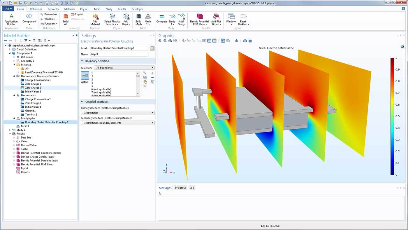
In addition to fundamental boundary conditions — such as potentials, currents, charges, and field values — a range of advanced boundary conditions are included. Some of these, including the Terminal, Floating Potential, and Circuit Terminal boundary conditions, are used to extract equivalent circuit parameters from a 2D or 3D model such as resistance, capacitance, inductance, and impedance values and matrices.
Boundary conditions in the AC/DC Module:
- Circuit Terminal
- Contact Resistance
- Dielectric Shielding
- Distributed Capacitance
- Distributed Impedance
- Distributed Resistance
- Electric Shielding
- Electrical Contact
- Lumped Port
- Periodic Boundary Condition
- Sector Symmetry
- Surface Impedance
- Surface Magnetic Current
- Thin Low Permeability Gap
- Transition
- Coil Excitation
- Homogenized Multiturn
- Single Conductor
- Floating Potential
- Magnetic Field
- Magnetic Flux Density
- Magnetic Insulation
- Magnetic Potential
- Perfect Magnetic Conductor
- Surface Current
- Boundary Current Source
- Continuity
- Displacement Field
- Electric Insulation
- Electric Potential
- Ground/Zero Potential
- Normal Current Density
- Surface Charge Density
- Zero Charge
- Magnetic Shielding
- B-H and H-B Curve Input
Modelling Thin Structures
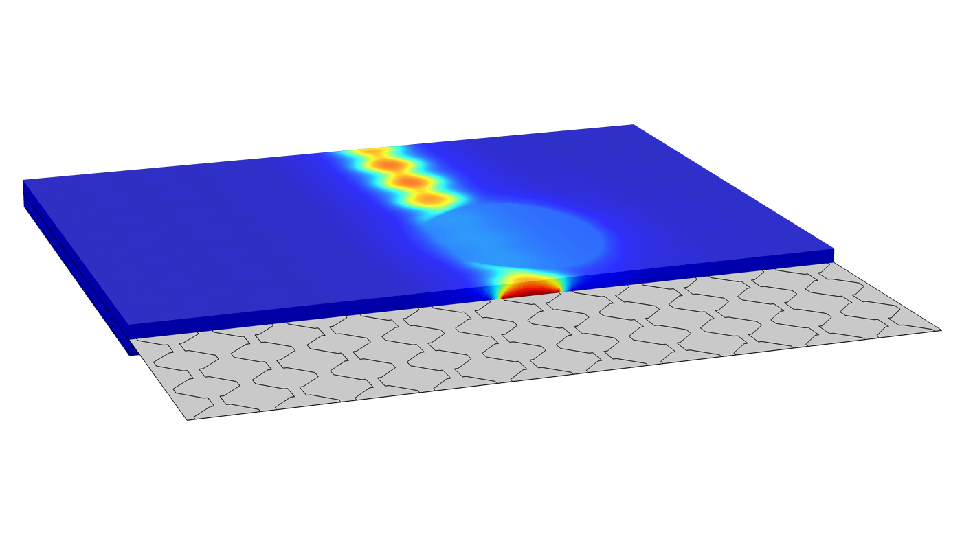
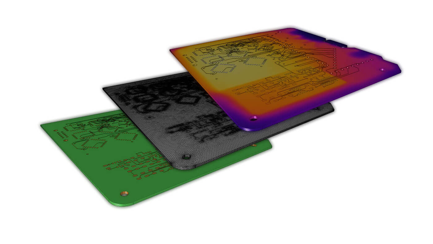
For modelling very thin structures, you can use shell formulations that are available for direct currents, electrostatics, magnetostatics, and induction simulations. A specialised user interface is available for modelling direct currents in shells with multiple layers. Electromagnetic shell modelling makes it possible to replace the thickness of a thin solid in a CAD model with a physical property of a surface resulting in a much more efficient representation.
Unbounded or Large Domains
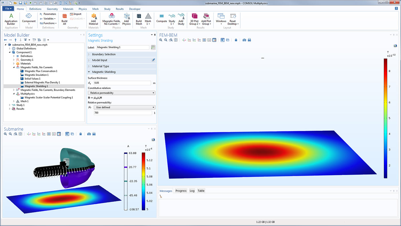
For accurate modelling of unbounded or large modelling domains, infinite elements are available for both electric and magnetic fields. For electrostatics and magnetostatics modelling, the boundary element method (BEM) is available as an alternative method for modelling large or infinite regions and works in combination with physics interfaces based on the finite element method (FEM).
Coil Modeling
Specialised coil features can be used to greatly simplify the setup process of coils for a range of magnetostatics and low-frequency electromagnetics models. In many such applications, the magnetic field is generated by electric currents flowing in conductive materials; for example, cables, wires, coils, or solenoids. The specialised coil features are used to easily model these structures and to translate lumped quantities, like currents and voltages, into distributed quantities, such as current densities and electric fields. Single-conductor and homogenised multiturn coils can be defined in full 3D or 2D axially symmetric models. A part library, with fully parametric coil and magnetic core shapes, enables faster model setup when analysing transformers, inductors, motors, and actuators.
Rotating Machinery and Linear Motion
Using the built-in interface for rotating machinery, it is easy to model motors and generators. You can, for example, understand the behaviour of induction or PM motors, particularly by capturing the eddy current losses that occur within the magnets. In any model that is used for simulating electromagnetic motion, you can examine the rigid or flexible body dynamics under the influence of magnetic forces and torques, induced currents, and mechanical load and spring configurations.
A general-purpose moving mesh functionality makes it possible to model linear motion. This is important for understanding the operation of components involving plungers, such as in magnetic power switches and general actuators.
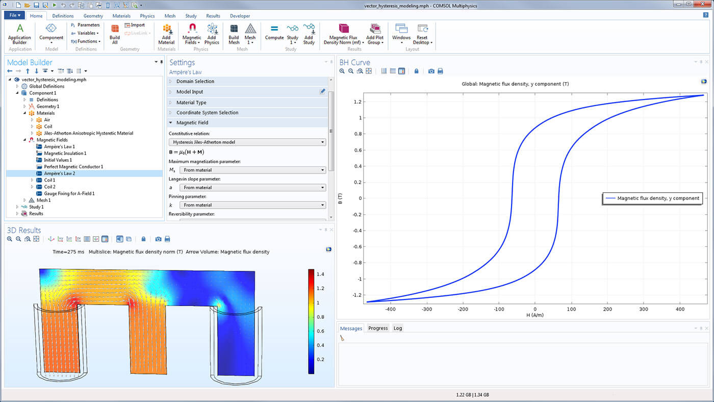
You can choose from a large material database that includes:
- Ferromagnetic materials
- Ferrimagnetic materials
- B-H curves
- H-B curves
In addition, you can use materials from libraries made available by other add-on products.
Materials can be spatially varying, anisotropic, time-varying, lossy, complex-valued, and discontinuous. It is easy to expand the scope of a simulation with little additional work. You can define your own materials using mathematical expressions, look-up tables, or combinations of both. Alternatively, you can use externally defined materials written in C-code.
More generally, by using the equation-based modelling functionality, you can modify boundary conditions, material properties, and equations to customise a simulation for your specific needs.
The AC/DC Module offers automatic, semiautomatic, and adaptive mesh generation. Under the hood, the AC/DC Module formulates and solves Maxwell’s equations using FEM, BEM, or a combination of both methods, in concert with state-of-the-art solvers. Several types of finite element and boundary element mesh elements are available.
Numerical methods in the AC/DC Module:
- FEM
- BEM
- Linear and high-order nodal-based and edge element discretisations
- Combinations of tetrahedral, prismatic, pyramidal, hexahedral, triangular, and quadrilateral elements
- Linear and nonlinear solvers
Study types in the AC/DC Module:
- Static
- Frequency domain
- Time domain
- Automated terminal sweeps for circuit parameter extraction
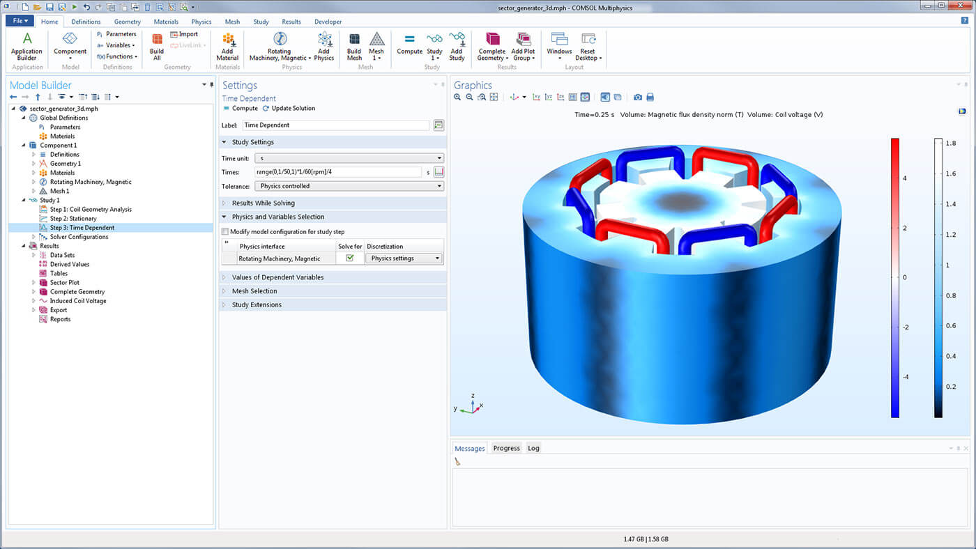
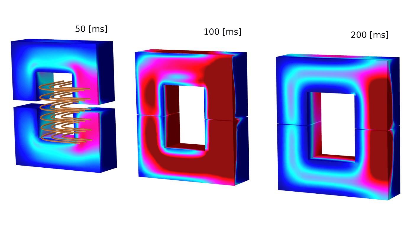
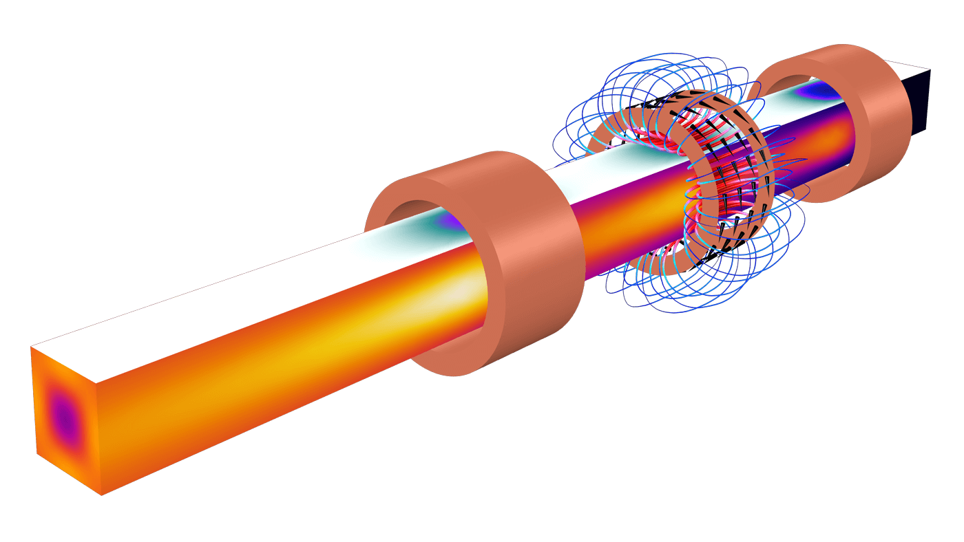
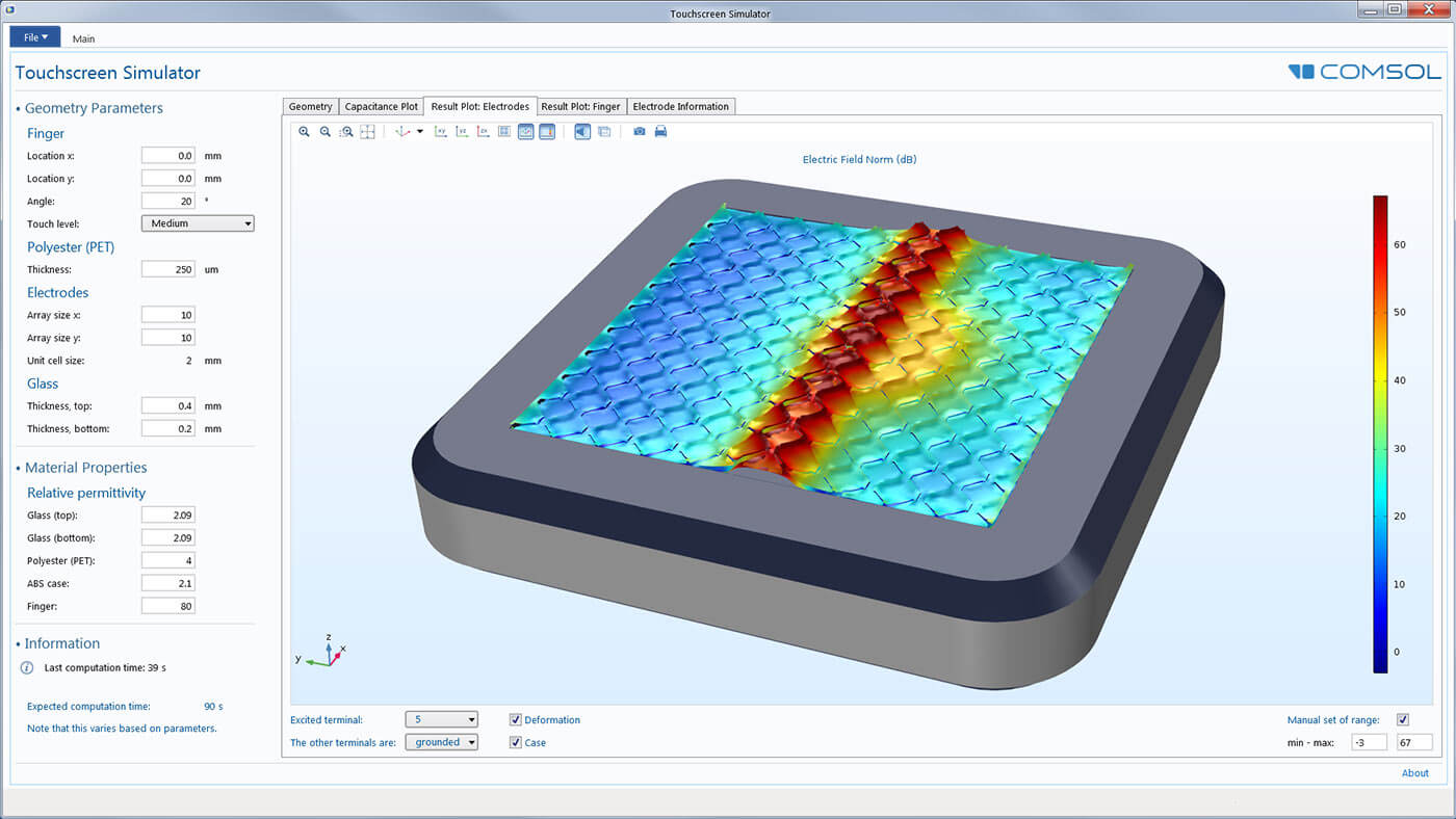
Default visualizations are automatically adapted to the interface you have used and include plots of electric and magnetic fields, currents, charges, and voltages. You can easily add custom visualizations of any field quantity as well as composite expressions of field quantities and their derivatives.
The postprocessing tools can be used to generate lumped parameter matrices, such as capacitance or impedance matrices, as well as integrated, averaged, maximum, and minimum values. For example, you can use a maximum field evaluation to make sure the dielectric strength is not exceeded anywhere in your model, or get the total charge by integrating the charge density over a set of surfaces. By using cut-lines and cut-surface, it is possible to examine the field values on arbitrary cross sections of a model.
Postprocessing and visualization features in the AC/DC Module:
- Voltage plots
- Electric field plots
- Magnetic field plots
- Current density plots
- Charge density plots
- Arbitrary expressions of physical quantities
- Derived tabulated quantities such as R-, L-, C-, Z-, Y-, and S-matrices
- Total charge and current
- Force and torque vs. time
 Tel: +61 (03) 6224 8690Email: info@technic.com.auConnect on LinkedInGet Your Free Trial